Marchenko redatuming by inversion

This example shows how to set-up and run the pylops_distributed.waveeqprocessing.Marchenko inversion using synthetic data.

Data are first converted to frequency domain and stored in the high-performance format Zarr. This allows lazy loading using a Dask array and distributing over frequencies the computation of the various Fredholm integrals involved in the forward model.

# sphinx_gallery_thumbnail_number = 3
import warnings
import numpy as np
import dask.array as da
import matplotlib.pyplot as plt

from scipy.signal import convolve
from pylops_distributed.waveeqprocessing import Marchenko

warnings.filterwarnings('ignore')
plt.close('all')

Let’s start by defining some input parameters and loading the test data

# Input parameters
inputfile = '../testdata/marchenko/input.npz'
inputzarr = '../testdata/marchenko/input.zarr'

vel = 2400.0         # velocity
toff = 0.045         # direct arrival time shift
nsmooth = 10         # time window smoothing
nfmax = 1000         # max frequency for MDC (#samples)
niter = 10           # iterations

inputdata = np.load(inputfile)

# Receivers
r = inputdata['r']
nr = r.shape[1]
dr = r[0, 1]-r[0, 0]

# Sources
s = inputdata['s']
ns = s.shape[1]
ds = s[0, 1]-s[0, 0]

# Virtual points
vs = inputdata['vs']

# Density model
rho = inputdata['rho']
z, x = inputdata['z'], inputdata['x']

# Reflection response in frequency domain (R[f, s, r])
R_fft = da.from_zarr(inputzarr)
print('R_fft:', R_fft)

# Subsurface fields
Gsub = inputdata['Gsub']
G0sub = inputdata['G0sub']
wav = inputdata['wav']
wav_c = np.argmax(wav)

t = inputdata['t']
ot, dt, nt = t[0], t[1]-t[0], len(t)

Gsub = np.apply_along_axis(convolve, 0, Gsub, wav, mode='full')
Gsub = Gsub[wav_c:][:nt]
G0sub = np.apply_along_axis(convolve, 0, G0sub, wav, mode='full')
G0sub = G0sub[wav_c:][:nt]

plt.figure(figsize=(10, 5))
plt.imshow(rho, cmap='gray', extent=(x[0], x[-1], z[-1], z[0]))
plt.scatter(s[0, 5::10], s[1, 5::10], marker='*', s=150, c='r', edgecolors='k')
plt.scatter(r[0, ::10], r[1, ::10], marker='v', s=150, c='b', edgecolors='k')
plt.scatter(vs[0], vs[1], marker='.', s=250, c='m', edgecolors='k')
plt.axis('tight')
plt.xlabel('x [m]')
plt.ylabel('y [m]')
plt.title('Model and Geometry')
plt.xlim(x[0], x[-1])

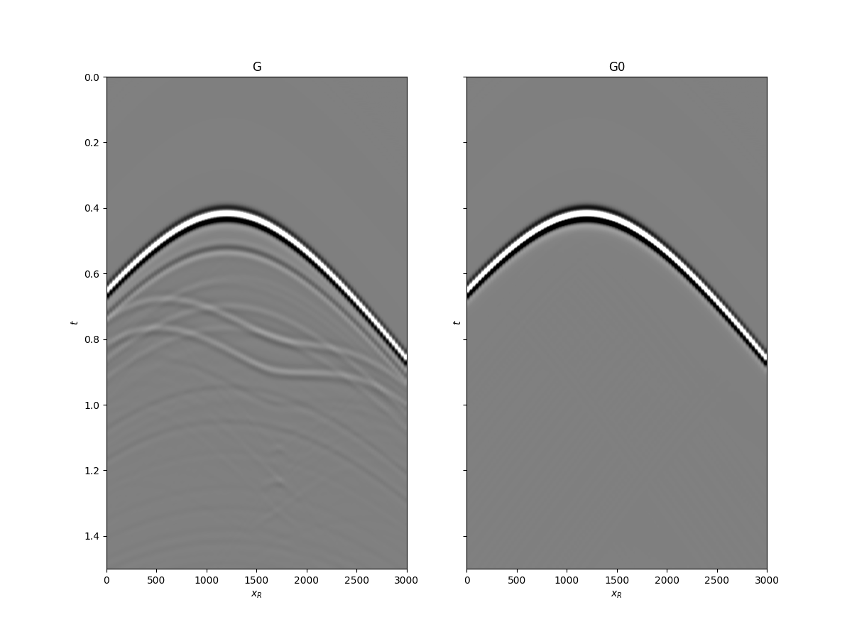
fig, axs = plt.subplots(1, 2, sharey=True, figsize=(12, 9))
axs[0].imshow(Gsub, cmap='gray', vmin=-1e6, vmax=1e6,
              extent=(r[0, 0], r[0, -1], t[-1], t[0]))
axs[0].set_title('G')
axs[0].set_xlabel(r'$x_R$')
axs[0].set_ylabel(r'$t$')
axs[0].axis('tight')
axs[0].set_ylim(1.5, 0)
axs[1].imshow(G0sub, cmap='gray', vmin=-1e6, vmax=1e6,
              extent=(r[0, 0], r[0, -1], t[-1], t[0]))
axs[1].set_title('G0')
axs[1].set_xlabel(r'$x_R$')
axs[1].set_ylabel(r'$t$')
axs[1].axis('tight')
axs[1].set_ylim(1.5, 0)

• 
• 

Out:

R_fft: dask.array<from-zarr, shape=(500, 101, 101), dtype=complex64, chunksize=(125, 101, 101), chunktype=numpy.ndarray>

(1.5, 0.0)

Let’s now create an object of the pylops_distributed.waveeqprocessing.Marchenko class and apply redatuming for a single subsurface point vs.

# direct arrival window
trav = np.sqrt((vs[0]-r[0])**2+(vs[1]-r[1])**2)/vel

MarchenkoWM = Marchenko(R_fft, nt=nt, dt=dt, dr=dr, wav=wav,
                        toff=toff, nsmooth=nsmooth)

f1_inv_minus, f1_inv_plus, p0_minus, g_inv_minus, g_inv_plus = \
    MarchenkoWM.apply_onepoint(trav, G0=G0sub.T, rtm=True, greens=True,
                               dottest=False, **dict(niter=niter, compute=True))
g_inv_tot = g_inv_minus + g_inv_plus

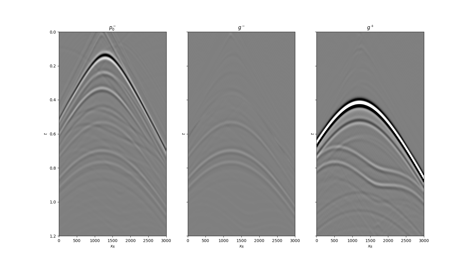
We can now compare the result of Marchenko redatuming via LSQR with standard redatuming

fig, axs = plt.subplots(1, 3, sharey=True, figsize=(16, 9))
axs[0].imshow(p0_minus.T, cmap='gray', vmin=-5e5, vmax=5e5,
              extent=(r[0, 0], r[0, -1], t[-1], -t[-1]))
axs[0].set_title(r'$p_0^-$')
axs[0].set_xlabel(r'$x_R$')
axs[0].set_ylabel(r'$t$')
axs[0].axis('tight')
axs[0].set_ylim(1.2, 0)
axs[1].imshow(g_inv_minus.T, cmap='gray', vmin=-5e5, vmax=5e5,
              extent=(r[0, 0], r[0, -1], t[-1], -t[-1]))
axs[1].set_title(r'$g^-$')
axs[1].set_xlabel(r'$x_R$')
axs[1].set_ylabel(r'$t$')
axs[1].axis('tight')
axs[1].set_ylim(1.2, 0)
axs[2].imshow(g_inv_plus.T, cmap='gray', vmin=-5e5, vmax=5e5,
              extent=(r[0, 0], r[0, -1], t[-1], -t[-1]))
axs[2].set_title(r'$g^+$')
axs[2].set_xlabel(r'$x_R$')
axs[2].set_ylabel(r'$t$')
axs[2].axis('tight')
axs[2].set_ylim(1.2, 0)

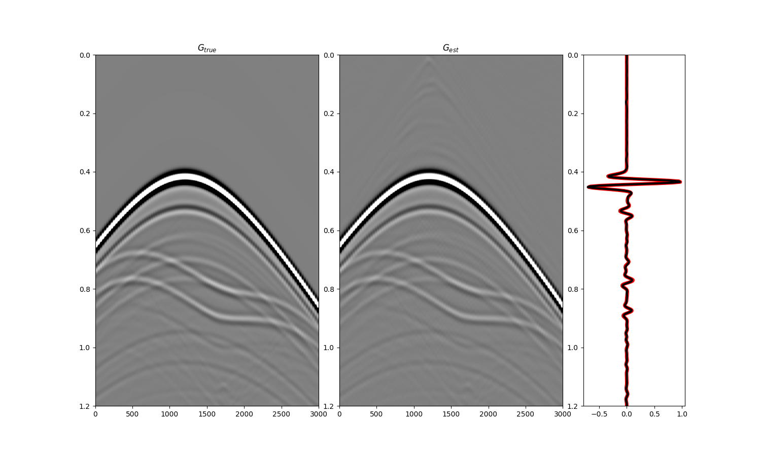
fig = plt.figure(figsize=(15, 9))
ax1 = plt.subplot2grid((1, 5), (0, 0), colspan=2)
ax2 = plt.subplot2grid((1, 5), (0, 2), colspan=2)
ax3 = plt.subplot2grid((1, 5), (0, 4))
ax1.imshow(Gsub, cmap='gray', vmin=-5e5, vmax=5e5,
           extent=(r[0, 0], r[0, -1], t[-1], t[0]))
ax1.set_title(r'$G_{true}$')
axs[0].set_xlabel(r'$x_R$')
axs[0].set_ylabel(r'$t$')
ax1.axis('tight')
ax1.set_ylim(1.2, 0)
ax2.imshow(g_inv_tot.T, cmap='gray', vmin=-5e5, vmax=5e5,
           extent=(r[0, 0], r[0, -1], t[-1], -t[-1]))
ax2.set_title(r'$G_{est}$')
axs[1].set_xlabel(r'$x_R$')
axs[1].set_ylabel(r'$t$')
ax2.axis('tight')
ax2.set_ylim(1.2, 0)
ax3.plot(Gsub[:, nr//2]/Gsub.max(), t, 'r', lw=5)
ax3.plot(g_inv_tot[nr//2, nt-1:]/g_inv_tot.max(), t, 'k', lw=3)
ax3.set_ylim(1.2, 0)

• 
• 

Out:

(1.2, 0.0)