09. Multi-Dimensional Deconvolution

This example shows how to set-up and run the pylops_distributed.waveeqprocessing.MDD inversion using synthetic data.

Data are first created as numpy arrays and then converted into Dask arrays. Data is chunked over frequencies to allow distributed computations of the Fredholm integral involved in the forward model.

NOTE: do not expect this code to run any fast than its pylops equivalent. for small datasets. The pylops-distributed framework should only be used when dealing with large datasets that do not fit in memory and benefit from distributed computing.

import warnings
import numpy as np
import dask.array as da
import matplotlib.pyplot as plt

from pylops.utils.tapers import taper3d
from pylops.utils.wavelets import ricker
from pylops.utils.seismicevents import makeaxis, hyperbolic2d
from pylops_distributed.waveeqprocessing import MDC, MDD

warnings.filterwarnings('ignore')
plt.close('all')

# sphinx_gallery_thumbnail_number = 3

Let’s start by creating a set of hyperbolic events to be used as our MDC kernel

# Input parameters
par = {'ox':-150, 'dx':10, 'nx':31,
       'oy':-250, 'dy':10, 'ny':51,
       'ot':0, 'dt':0.004, 'nt':300,
       'f0': 20, 'nfmax': 200}

t0_m = [0.2]
vrms_m = [700.]
amp_m = [1.]

t0_G = [0.2, 0.5, 0.7]
vrms_G = [800., 1200., 1500.]
amp_G = [1., 0.6, 0.5]

# Taper
tap = taper3d(par['nt'], [par['ny'], par['nx']],
              (5, 5), tapertype='hanning')

# Create axis
t, t2, x, y = makeaxis(par)

# Create wavelet
wav = ricker(t[:41], f0=par['f0'])[0]

# Generate model
m, mwav = hyperbolic2d(x, t, t0_m, vrms_m, amp_m, wav)

# Generate operator
G, Gwav = np.zeros((par['ny'], par['nx'], par['nt'])), \
          np.zeros((par['ny'], par['nx'], par['nt']))
for iy, y0 in enumerate(y):
    G[iy], Gwav[iy] = hyperbolic2d(x-y0, t, t0_G, vrms_G, amp_G, wav)
G, Gwav = G*tap, Gwav*tap

# Add negative part to data and model
m = np.concatenate((np.zeros((par['nx'], par['nt']-1)), m), axis=-1)
mwav = np.concatenate((np.zeros((par['nx'], par['nt']-1)), mwav), axis=-1)
Gwav2 = np.concatenate((np.zeros((par['ny'], par['nx'], par['nt']-1)), Gwav),
                       axis=-1)

# Define MDC linear operator
Gwav_fft = np.fft.rfft(Gwav2, 2*par['nt']-1, axis=-1)
Gwav_fft = Gwav_fft[..., :par['nfmax']]
Gwav_fft = np.transpose(Gwav_fft, (2, 0, 1))

# Convert inputs to Dask and chunk frequency axis in 4 equal parts
m = da.from_array(m.T, chunks=(2*par['nt']-1, par['nx'])).ravel()
Gwav_fft = da.from_array(Gwav_fft, chunks=(par['nfmax'] // 4,
                                           par['ny'], par['nx']))
print(Gwav_fft)

# Define MDC linear operator
MDCop = MDC(Gwav_fft, nt=2 * par['nt']-1, nv=1)

# Create data
d = MDCop * m.flatten()
d = d.reshape(2*par['nt']-1, par['ny'])

Out:

dask.array<array, shape=(200, 51, 31), dtype=complex128, chunksize=(50, 51, 31), chunktype=numpy.ndarray>

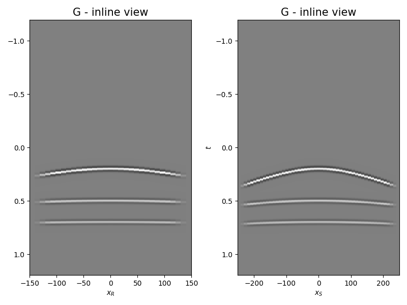
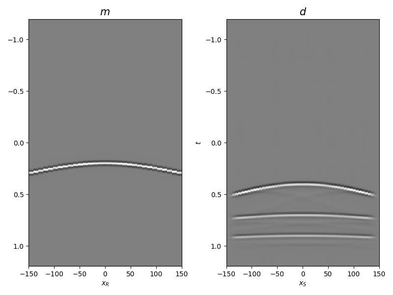
Let’s display what we have so far: operator, input model, and data

fig, axs = plt.subplots(1, 2, figsize=(8, 6))
axs[0].imshow(Gwav2[int(par['ny']/2)].T, aspect='auto',
              interpolation='nearest', cmap='gray',
              vmin=-np.abs(Gwav2.max()), vmax=np.abs(Gwav2.max()),
              extent=(x.min(), x.max(), t2.max(), t2.min()))
axs[0].set_title('G - inline view', fontsize=15)
axs[0].set_xlabel(r'$x_R$')
axs[1].set_ylabel(r'$t$')
axs[1].imshow(Gwav2[:, int(par['nx']/2)].T, aspect='auto',
              interpolation='nearest', cmap='gray',
              vmin=-np.abs(Gwav2.max()), vmax=np.abs(Gwav2.max()),
              extent=(y.min(), y.max(), t2.max(), t2.min()))
axs[1].set_title('G - inline view', fontsize=15)
axs[1].set_xlabel(r'$x_S$')
axs[1].set_ylabel(r'$t$')
fig.tight_layout()

fig, axs = plt.subplots(1, 2, figsize=(8, 6))
axs[0].imshow(mwav.T, aspect='auto', interpolation='nearest', cmap='gray',
              vmin=-np.abs(mwav.max()), vmax=np.abs(mwav.max()),
              extent=(x.min(), x.max(), t2.max(), t2.min()))
axs[0].set_title(r'$m$', fontsize=15)
axs[0].set_xlabel(r'$x_R$')
axs[1].set_ylabel(r'$t$')
axs[1].imshow(d, aspect='auto', interpolation='nearest', cmap='gray',
              vmin=-np.abs(d.max()), vmax=np.abs(d.max()),
              extent=(x.min(), x.max(), t2.max(), t2.min()))
axs[1].set_title(r'$d$', fontsize=15)
axs[1].set_xlabel(r'$x_S$')
axs[1].set_ylabel(r'$t$')
fig.tight_layout()

• 
• 

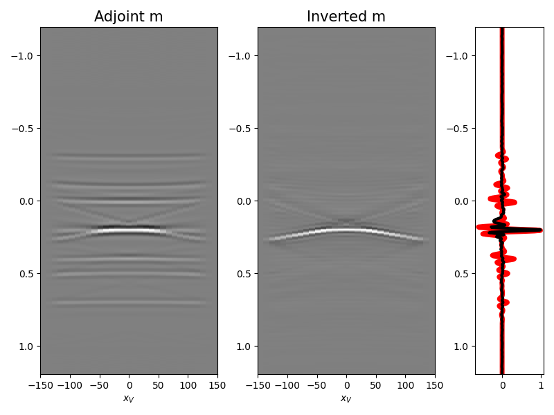
We are now ready to feed our operator to pylops.waveeqprocessing.MDD and invert back for our input model

minv, madj = MDD(Gwav_fft, d[par['nt'] - 1:],
                 dt=par['dt'], dr=par['dx'],
                 nfmax=par['nfmax'], wav=wav,
                 twosided=True, add_negative=True,
                 adjoint=True, dottest=False,
                 **dict(niter=10, compute=False))

fig = plt.figure(figsize=(8, 6))
ax1 = plt.subplot2grid((1, 5), (0, 0), colspan=2)
ax2 = plt.subplot2grid((1, 5), (0, 2), colspan=2)
ax3 = plt.subplot2grid((1, 5), (0, 4))
ax1.imshow(madj, aspect='auto', interpolation='nearest', cmap='gray',
           vmin=-np.abs(madj.max()), vmax=np.abs(madj.max()),
           extent=(x.min(), x.max(), t2.max(), t2.min()))
ax1.set_title('Adjoint m', fontsize=15)
ax1.set_xlabel(r'$x_V$')
axs[1].set_ylabel(r'$t$')
ax2.imshow(minv, aspect='auto', interpolation='nearest', cmap='gray',
           vmin=-np.abs(minv.max()), vmax=np.abs(minv.max()),
           extent=(x.min(), x.max(), t2.max(), t2.min()))
ax2.set_title('Inverted m', fontsize=15)
ax2.set_xlabel(r'$x_V$')
axs[1].set_ylabel(r'$t$')
ax3.plot(madj[:, int(par['nx']/2)]/np.abs(madj[:, int(par['nx']/2)]).max(),
         t2, 'r', lw=5)
ax3.plot(minv[:, int(par['nx']/2)]/np.abs(minv[:, int(par['nx']/2)]).max(),
         t2, 'k', lw=3)
ax3.set_ylim([t2[-1], t2[0]])
fig.tight_layout()