Marchenko redatuming by inversion

This example shows how to set-up and run the pylops_distributed.waveeqprocessing.Marchenko inversion using synthetic data.

Data are first converted to frequency domain and stored in the high-performance format Zarr. This allows lazy loading using a Dask array and distributing over frequencies the computation of the various Fredholm integrals involved in the forward model.

NOTE: do not expect this code to run any fast than its pylops equivalent. for small datasets. The pylops-distributed framework should only be used when dealing with large datasets that do not fit in memory and benefit from distributed computing.

import warnings
import numpy as np
import dask.array as da
import matplotlib.pyplot as plt

from scipy.signal import convolve
from pylops_distributed.waveeqprocessing import Marchenko

warnings.filterwarnings('ignore')
plt.close('all')

# sphinx_gallery_thumbnail_number = 4

Let’s start by defining some input parameters and loading the test data

# Input parameters
inputfile = '../testdata/marchenko/input.npz'
inputzarr = '../testdata/marchenko/input.zarr'

vel = 2400.0         # velocity
toff = 0.045         # direct arrival time shift
nsmooth = 10         # time window smoothing
nfmax = 1000         # max frequency for MDC (#samples)
niter = 10           # iterations

inputdata = np.load(inputfile)

# Receivers
r = inputdata['r']
nr = r.shape[1]
dr = r[0, 1]-r[0, 0]

# Sources
s = inputdata['s']
ns = s.shape[1]
ds = s[0, 1]-s[0, 0]

# Virtual points
vs = inputdata['vs']

# Density model
rho = inputdata['rho']
z, x = inputdata['z'], inputdata['x']

# Reflection response in frequency domain (R[f, s, r])
R_fft = da.from_zarr(inputzarr)
print('R_fft:', R_fft)

# Subsurface fields
Gsub = inputdata['Gsub']
G0sub = inputdata['G0sub']
wav = inputdata['wav']
wav_c = np.argmax(wav)

t = inputdata['t']
ot, dt, nt = t[0], t[1]-t[0], len(t)

Gsub = np.apply_along_axis(convolve, 0, Gsub, wav, mode='full')
Gsub = Gsub[wav_c:][:nt]
G0sub = np.apply_along_axis(convolve, 0, G0sub, wav, mode='full')
G0sub = G0sub[wav_c:][:nt]

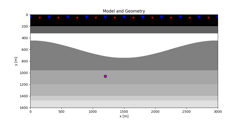
plt.figure(figsize=(10, 5))
plt.imshow(rho, cmap='gray', extent=(x[0], x[-1], z[-1], z[0]))
plt.scatter(s[0, 5::10], s[1, 5::10], marker='*', s=150, c='r', edgecolors='k')
plt.scatter(r[0, ::10], r[1, ::10], marker='v', s=150, c='b', edgecolors='k')
plt.scatter(vs[0], vs[1], marker='.', s=250, c='m', edgecolors='k')
plt.axis('tight')
plt.xlabel('x [m]')
plt.ylabel('y [m]')
plt.title('Model and Geometry')
plt.xlim(x[0], x[-1])

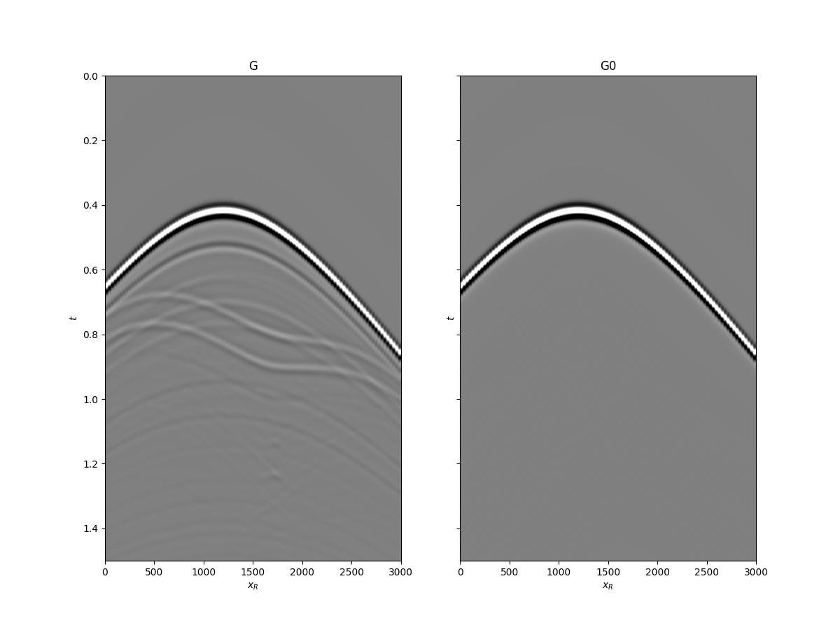
fig, axs = plt.subplots(1, 2, sharey=True, figsize=(12, 9))
axs[0].imshow(Gsub, cmap='gray', vmin=-1e6, vmax=1e6,
              extent=(r[0, 0], r[0, -1], t[-1], t[0]))
axs[0].set_title('G')
axs[0].set_xlabel(r'$x_R$')
axs[0].set_ylabel(r'$t$')
axs[0].axis('tight')
axs[0].set_ylim(1.5, 0)
axs[1].imshow(G0sub, cmap='gray', vmin=-1e6, vmax=1e6,
              extent=(r[0, 0], r[0, -1], t[-1], t[0]))
axs[1].set_title('G0')
axs[1].set_xlabel(r'$x_R$')
axs[1].set_ylabel(r'$t$')
axs[1].axis('tight')
axs[1].set_ylim(1.5, 0)

• 
• 

Out:

R_fft: dask.array<from-zarr, shape=(500, 101, 101), dtype=complex64, chunksize=(125, 101, 101), chunktype=numpy.ndarray>

(1.5, 0.0)

Let’s now create an object of the pylops_distributed.waveeqprocessing.Marchenko class and apply redatuming for a single subsurface point vs.

# direct arrival window
trav = np.sqrt((vs[0]-r[0])**2+(vs[1]-r[1])**2)/vel

MarchenkoWM = Marchenko(R_fft, nt=nt, dt=dt, dr=dr, wav=wav,
                        toff=toff, nsmooth=nsmooth)

f1_inv_minus, f1_inv_plus, p0_minus, g_inv_minus, g_inv_plus = \
    MarchenkoWM.apply_onepoint(trav, G0=G0sub.T, rtm=True, greens=True,
                               dottest=False, **dict(niter=niter, compute=True))
g_inv_tot = g_inv_minus + g_inv_plus

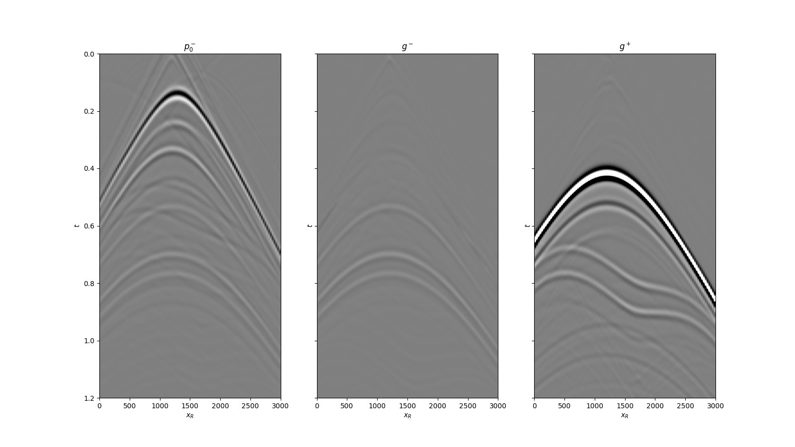
We can now compare the result of Marchenko redatuming via LSQR with standard redatuming

fig, axs = plt.subplots(1, 3, sharey=True, figsize=(16, 9))
axs[0].imshow(p0_minus.T, cmap='gray', vmin=-5e5, vmax=5e5,
              extent=(r[0, 0], r[0, -1], t[-1], -t[-1]))
axs[0].set_title(r'$p_0^-$')
axs[0].set_xlabel(r'$x_R$')
axs[0].set_ylabel(r'$t$')
axs[0].axis('tight')
axs[0].set_ylim(1.2, 0)
axs[1].imshow(g_inv_minus.T, cmap='gray', vmin=-5e5, vmax=5e5,
              extent=(r[0, 0], r[0, -1], t[-1], -t[-1]))
axs[1].set_title(r'$g^-$')
axs[1].set_xlabel(r'$x_R$')
axs[1].set_ylabel(r'$t$')
axs[1].axis('tight')
axs[1].set_ylim(1.2, 0)
axs[2].imshow(g_inv_plus.T, cmap='gray', vmin=-5e5, vmax=5e5,
              extent=(r[0, 0], r[0, -1], t[-1], -t[-1]))
axs[2].set_title(r'$g^+$')
axs[2].set_xlabel(r'$x_R$')
axs[2].set_ylabel(r'$t$')
axs[2].axis('tight')
axs[2].set_ylim(1.2, 0)

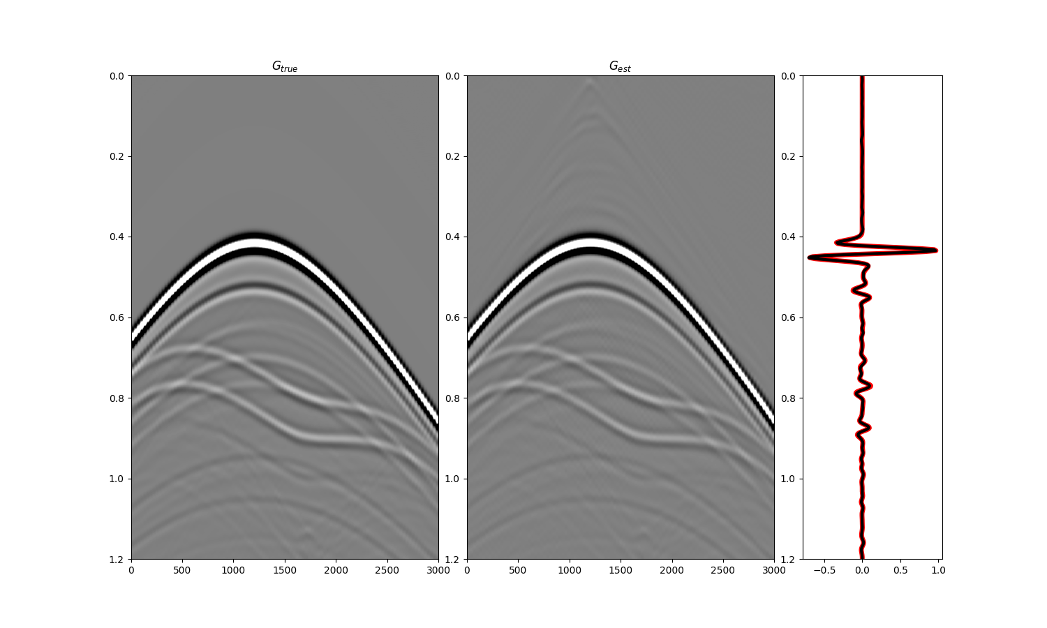
fig = plt.figure(figsize=(15, 9))
ax1 = plt.subplot2grid((1, 5), (0, 0), colspan=2)
ax2 = plt.subplot2grid((1, 5), (0, 2), colspan=2)
ax3 = plt.subplot2grid((1, 5), (0, 4))
ax1.imshow(Gsub, cmap='gray', vmin=-5e5, vmax=5e5,
           extent=(r[0, 0], r[0, -1], t[-1], t[0]))
ax1.set_title(r'$G_{true}$')
axs[0].set_xlabel(r'$x_R$')
axs[0].set_ylabel(r'$t$')
ax1.axis('tight')
ax1.set_ylim(1.2, 0)
ax2.imshow(g_inv_tot.T, cmap='gray', vmin=-5e5, vmax=5e5,
           extent=(r[0, 0], r[0, -1], t[-1], -t[-1]))
ax2.set_title(r'$G_{est}$')
axs[1].set_xlabel(r'$x_R$')
axs[1].set_ylabel(r'$t$')
ax2.axis('tight')
ax2.set_ylim(1.2, 0)
ax3.plot(Gsub[:, nr//2]/Gsub.max(), t, 'r', lw=5)
ax3.plot(g_inv_tot[nr//2, nt-1:]/g_inv_tot.max(), t, 'k', lw=3)
ax3.set_ylim(1.2, 0)

• 
• 

Out:

(1.2, 0.0)