Restriction

This example shows how to use the pylops_distributed.Restriction operator to sample a certain input vector at desired locations iava.

import numpy as np
import matplotlib.pyplot as plt
import dask.array as da
import pylops_distributed

plt.close('all')
np.random.seed(10)

Let’s create a signal of size nt and sampling dt that is composed of three sinusoids at frequencies freqs.

nt = 200
dt = 0.004

freqs = [5., 3., 8.]

t = np.arange(nt)*dt
x = np.zeros(nt)

for freq in freqs:
    x = x + np.sin(2*np.pi*freq*t)
x = da.from_array(x, chunks=(nt//4))

First of all, we subsample the signal at random locations and we retain 40% of the initial samples.

perc_subsampling = 0.4
ntsub = int(np.round(nt*perc_subsampling))

isample = np.arange(nt)
iava = np.sort(np.random.permutation(np.arange(nt))[:ntsub])

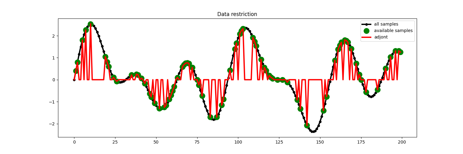
We then create the restriction and interpolation operators and display the original signal as well as the subsampled signal.

Rop = pylops_distributed.Restriction(nt, iava, dtype='float64',
                                     compute=(False, False))


y = Rop * x
xadj = Rop.H * y

# Visualize data
fig = plt.figure(figsize=(15, 5))
plt.plot(isample, x, '.-k', lw=3, ms=10, label='all samples')
plt.plot(iava, y, '.g', ms=25, label='available samples')
plt.plot(isample, xadj, 'r', lw=3, label='adjont')
plt.legend()
plt.title('Data restriction')

Out:

Text(0.5, 1.0, 'Data restriction')

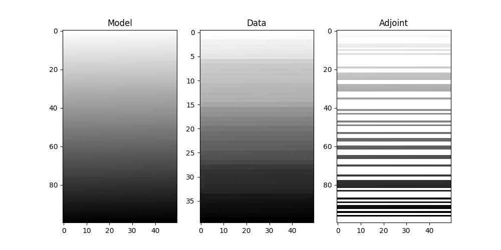
Finally we show how the pylops.Restriction is not limited to one dimensional signals but can be applied to sample locations of a specific axis of a multi-dimensional array. subsampling locations

nx, nt = 100, 50

x = np.arange(nx*nt).reshape(nx, nt)
x = da.from_array(x, chunks=(nx//4, nt//2))

perc_subsampling = 0.4
nxsub = int(np.round(nx*perc_subsampling))
iava = np.sort(np.random.permutation(np.arange(nx))[:nxsub])

Rop = pylops_distributed.Restriction(nx*nt, iava, dims=(nx, nt), dir=0,
                                     dtype='float64', compute=(False, False))

y = (Rop * x.ravel()).reshape(nxsub, nt)
xadj = (Rop.H * y.ravel()).reshape(nx, nt)

fig, axs = plt.subplots(1, 3, figsize=(10, 5))
axs[0].imshow(x, cmap='gray_r')
axs[0].set_title('Model')
axs[0].axis('tight')
axs[1].imshow(y, cmap='gray_r')
axs[1].set_title('Data')
axs[1].axis('tight')
axs[2].imshow(xadj, cmap='gray_r')
axs[2].set_title('Adjoint')
axs[2].axis('tight')

Out:

(-0.5, 49.5, 99.5, -0.5)